Forecast Center

November/December 2009

by TIM VASQUEZ / www.weathergraphics.com

This article is a courtesy copy placed on the author's website for educational purposes as permitted by written agreement with Taylor & Francis. It may not be distributed or reproduced without express written permission of Taylor & Francis. More recent installments of this article may be found at the link which follows. Publisher's Notice: This is a preprint of an article submitted for consideration in Weatherwise © 2009 Copyright Taylor & Francis. Weatherwise magazine is available online at: http://www.informaworld.com/openurl?genre=article&issn=0043-1672&volume=62&issue=6&spage=66.

PART ONE: The Puzzle

For meteorologists, autumn marks the start of a turbulent time for forecasters. Solar heating is reduced and powerful cold air masses begin to form in polar regions. When these cold air masses move into temperate regions, mingling with warm ground and ocean surfaces, they are heated from below and quickly destabilize, producing gusty winds and cumuliform clouds. The leading edge of these cold air masses produces strong zones of wind convergence, so squall lines and organized thunderstorms become much more common. But in most cases, cold air reaches the United States in weak southward thrusts. In this puzzle, we'll take a look at such an example, illustrating a pattern commonly seen by forecasters in September and October.

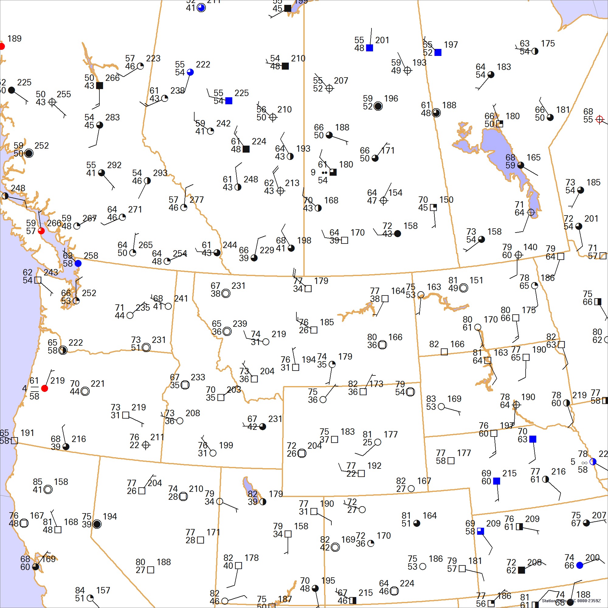
This weather map depicts a weather situation at midday in September. Draw isobars every four millibars (996, 1000, 1004 mb, etc) using the plot model example at the lower right as a guide. As the plot model indicates, the actual millibar value for plotted pressure (xxx) is 10xx.x mb when the number shown is below 500, and 9xx.x when it is more than 500. For instance, 027 represents 1002.7 mb and 892 represents 989.2 mb. Therefore, when one station reports 074 and a nearby one shows 086, the 1008 mb isobar will be found halfway between the stations. Then try to find the locations of fronts, highs, and lows.

Click to enlarge

* * * * *

Scroll down for the solution

* * * * *

PART TWO: The Solution

Autumn brings the arrival of fast-moving, benign systems that bring cold, dry Canadian air masses originating from the interior regions of Canada. These are known informally as Alberta clippers. Though cold fronts are common year-round in the northern tier states, the first true Alberta clippers appear in September and become more common in October and November. They differ from Pacific systems, which originate from the West Coast and tend to bring weaker temperature drops but stronger upper-level support with more organized precipitation areas. Alberta clippers are popularly associated with modest temperature drops, gusty wind, and brief precipitation, but more powerful, organized ones with large precipitation areas are known to forecasters simply as "polar outbreaks" or simply the unambiguous phrase "cold front".

This issue's map shows the weather at about 12 noon local time on September 10, 2009. A strong cold front is the most noticeable feature, extending from Saskatchewan through Montana with no significant weather except for strong winds and cool temperatures in its wake. The cold front is being driven by a 1029 mb high pressure area over British Columbia, advecting cold air southward through Alberta into Montana.

What causes the strong winds? It's due to the strong pressure gradient, or difference in pressure per unit distance, revealed by the close isobar spacing in Montana, Alberta, and Saskatchewan. Though wind gusts are not marked on this map, these winds behind the front are quite gusty. The gustiness is caused by heating of the cold air mass over the warm land mass. This causes the cool air mass to become unstable, since the warm ground adds buoyancy to the lower layers of this air. The result is a churning of the air as it expends this added buoyant energy and equalizes its temperature characteristics through the vertical. This process, known as mixing, brings gusty winds, turbulence, and if enough moisture is present, cumulus and stratocumulus clouds.

Also shown on the chart are a series of troughs extending from the Dakotas to Colorado and Utah. This has been accentuated by drawing the 1018 mb isobar. Though the puzzle didn't call for it, there is no rule against adding extra contours, and forecasters are always encouraged to add features and markings that help bring understanding to the analysis. Since there are no significant temperature contrasts across this zone, it is not a "baroclinic", or frontal feature. So it is drawn as a trough. These troughs in warm air mass regions tend to coincide with the axis of warmest temperatures and strongest heating, as revealed here by the near-80 degree temperature readings along much of its length. This is also the cause of the lows shown in California. Troughs near mountain ranges can often be amplified by "lee side troughing", which occurs when strong westerly winds cross the Rocky Mountains, producing low pressure east of the mountains due to conservation of angular momentum, or the "ice skater effect", is the column of air stretches vertically with the ground falling away beneath.

With the high pressure area appearing to extend all the way from British Columbia to Nevada and Utah, it may be tempting for many readers to draw the cold front all the way south to Utah and Nevada. In fact, I considered this possibility carefully while preparing this puzzle due to the weak north winds in Oregon. However there are no sharp temperature contrasts anywhere from Las Vegas to Washington state. Familiarity with the climate is also helpful. The normal high temperature in Seattle in September is 69 degrees and in Spokane is 72. The puzzle is for noon and the temperatures are already near those levels, so the day's temperatures are at or above normal. The cool readings in southwest Oregon may be deceptive, entirely due to the overcast clouds at those locations. So here, the cool air action is focused mostly in Montana, Saskatchewan, and Alberta.

Computers do not produce the puzzle solution. The weather chart is created automatically with Digital Atmosphere, but fronts and isobars are added by hand using Adobe Illustrator.