Forecast Center

January/February 2010

by TIM VASQUEZ / www.weathergraphics.com

This article is a courtesy copy placed on the author's website for educational purposes as permitted by written agreement with Taylor & Francis. It may not be distributed or reproduced without express written permission of Taylor & Francis. More recent installments of this article may be found at the link which follows. Publisher's Notice: This is a preprint of an article submitted for consideration in Weatherwise © 2010 Copyright Taylor & Francis. Weatherwise magazine is available online at: http://www.informaworld.com/openurl?genre=article&issn=0043-1672&volume=63&issue=1&spage=70.

PART ONE: The Puzzle

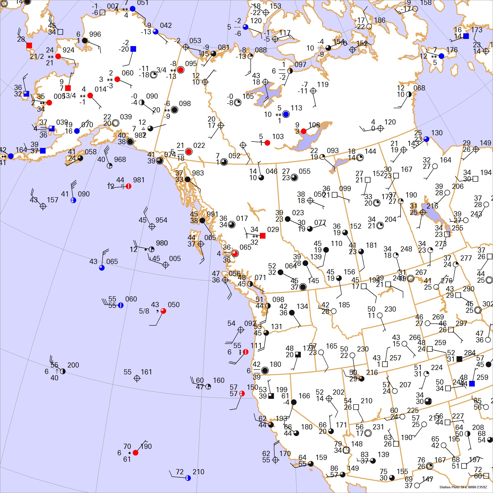
Now that North America is in the depths of winter, it's perhaps appropriate to take a closer look at the weather in Alaska, the northern Pacific, and western Canada. All of these regions have a major effect on the weather in North America. There are a number of fronts in this puzzle, but they will be a challenge to find. The key is in careful placement of isobars and attention to the weather patterns shown at various stations on the map. In the western United States, where terrain frequently disrupts horizontal constency of the analysis, it's especially helpful to identify some of the stations and compare the conditions against climatological normals.

This weather map depicts a weather situation in midafternoon in November. Draw isobars every four millibars (996, 1000, 1004 mb, etc) using the plot model example at the lower right as a guide. As the plot model indicates, the actual millibar value for plotted pressure (xxx) is 10xx.x mb when the number shown is below 500, and 9xx.x when it is more than 500. For instance, 027 represents 1002.7 mb and 892 represents 989.2 mb. Therefore, when one station reports 074 and a nearby one shows 086, the 1008 mb isobar will be found halfway between the stations. Then try to find the locations of fronts, highs, and lows.

Click to enlarge

* * * * *

Scroll down for the solution

* * * * *

PART TWO: The Solution

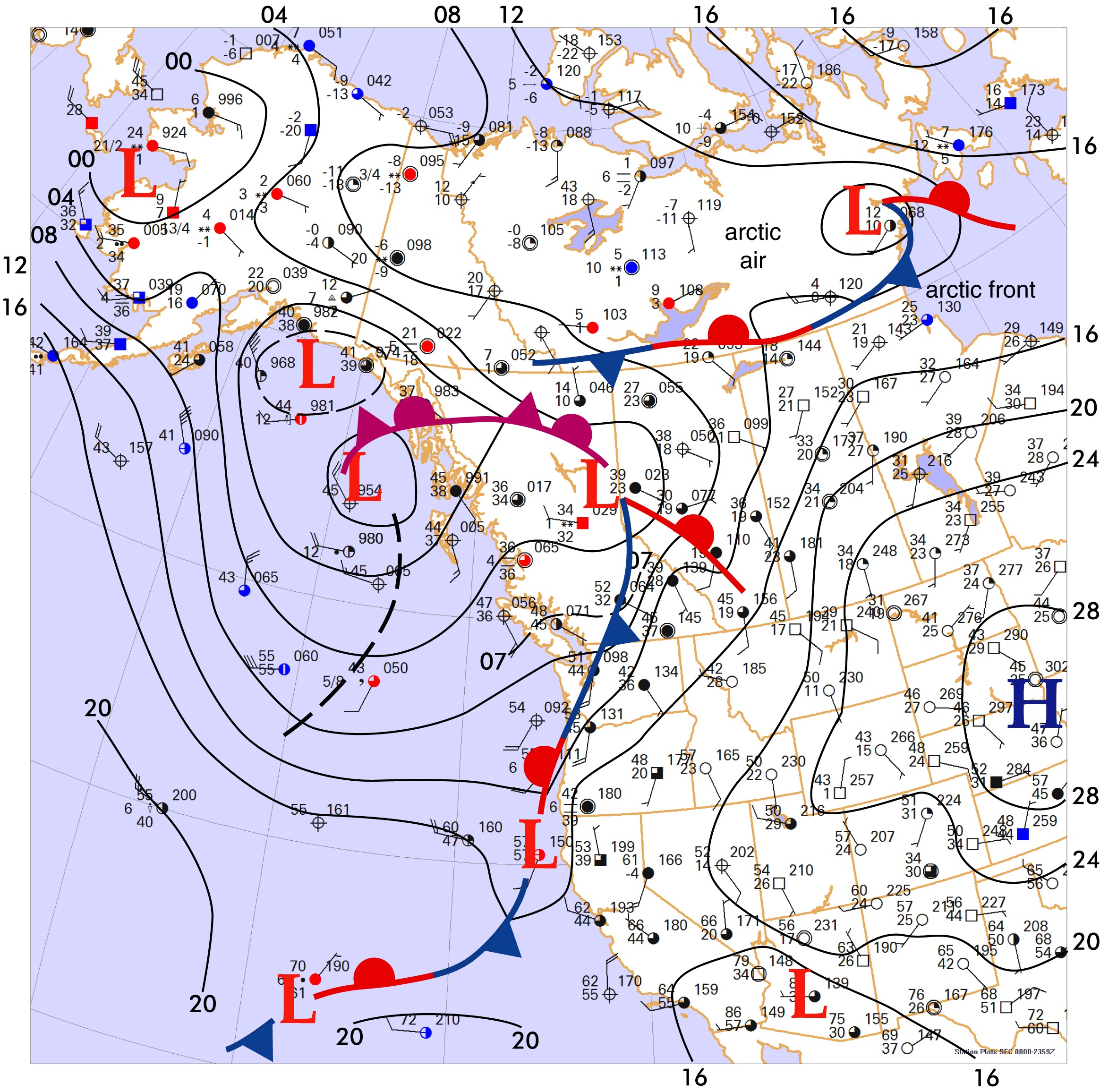
While the isobars may be easy for anyone who sketches them methodically and attentively, the location of the fronts makes this panel among of the more challenging puzzles we've printed. Some readers may have found different placements, but small differences are acceptable, and if there is good reason for them it may even demonstrate acute awareness of noteworthy meteorological features. Hand analysis is often misunderstood as a chart coloring exercise when in fact it is a technique that gives the forecaster a coherent understanding of the weather conditions across an area. Highlighting features and questioning why they exist goes much further towards building forecast wisdom than seeking markings that demonstrate cookie-cutter conformity!

In drawing this solution for the afternoon of November 9, 2009, the deep low near the Gulf of Alaska and the sharp troughing down the west coast depicts a classic pattern of a frontal system coming ashore. I initially connected the Pacific coast front into the low off the British Columbia coast, assuming it was an occluded system. But after a few minutes of thought I erased this and connected the front further eastward in British Columbia. Why? While I was drawing isobars I noticed the low pressure area in east central British Columbia, which showed cyclonic rotation, snow, and low clouds. This is not the type of organized system that should be normally be found ahead of a frontal system. After examining it further I decided that it had to be the "real" frontal low.

The lows in the Gulf of Alaska, therefore, are back in the cold air, disconnected from the frontal systems, and are old decaying occluded lows. Note how frigid air from the Alaskan interior advects southward over the warmer ocean waters. When very cold air masses like this are heated strongly from below, it promotes a cold-over-warm atmospheric profile, the exact definition of instability. This promotes a vigorous churning motion in the low-levels of the atmosphere, producing very gusty winds and, if the unstable layer is deep enough, snow showers or rain showers. This type of weather is the chief hazard to Alaskan offshore fishing operations: the peak of crab season is November and December!

Now that a frontal system has been identified, the next question is, "Where is the warm front?" After all, drawing a cold front means that there is a division between cold and warm air. Warm air usually enters a frontal system in the form of a wedge or a tongue, and marking a cold front only delineates one edge of it. By examining the warm sector, we figure how far north the warm air extends, where the warm front is, and if part of the cold front is actually occluded.

Unfortunately, the warm air primarily covers the western United States, which is quite rugged with weather stations at many different elevations. Not only is it difficult to compare two stations due to the difference in altitude but weather may be affected by terrain, a classic example being a station trapped in a valley which fails to break out of a foggy pattern. Normally forecasters monitor trends, but continuity is not available with a single weather map. A different technique is called for. Climatology normals, which are widely found on the Internet, are just what's called for. For example, Reno shows 61 degrees, but considered against Reno's normal high for November of 55 the station is clearly warmer than normal. North through Idaho temperatures are well above normal. Even Montana and Alberta are above normal, but here the temperatures are biased by adiabatic warming due to the southerly and southwesterly winds. I reluctantly placed the warm front as shown, essentially placing it in the lee side trough as it appeared that the two were colocated.

This left the task of correctly positioning the front through Washington and British Columbia, especially since it must always lie in a trough. I found it helpful to draw an intermediate isobar, that is, an isobar that is not normally called for. I selected the 1007 mb line and drew it in a dashed line as shown. This revealed an area of troughing east of Vancouver. I then used this to refine the position of the frontal system. Further down the front, the nearly closed isobars suggest waves along the front and possible low pressure areas, as shown. The data does not actually support these lows and they are hypothesized, so it is perfectly acceptable if they're omitted and the front simply shown as an undulating stable wave.

The last feature worth mentioning is the weak frontal system in the Canadian arctic. This separates cool 30s air from very cold near-zero conditions. This is in fact the arctic front, and the air poleward of it consists largely of stagnant air above snow cover. The arctic air mass has a tendency to radiate away heat into space and grow colder with time. If the depth of the arctic air builds and northwesterly upper-level flow develops, it may send severe outbreaks of cold air southward into southern Canada and the United States, especially during the weeks spanning late December through early February.

Computers do not produce the puzzle solution. The weather chart is created automatically with Digital Atmosphere, but fronts and isobars are added by hand using Adobe Illustrator.