Forecast Center

March/April 2009

by TIM VASQUEZ / www.weathergraphics.com

This article is a courtesy copy placed on the author's website for educational purposes as permitted by written agreement with Taylor & Francis. It may not be distributed or reproduced without express written permission of Taylor & Francis. More recent installments of this article may be found at the link which follows. Publisher's Notice: This is a preprint of an article submitted for consideration in Weatherwise 짤 2009 Copyright Taylor & Francis. Weatherwise magazine is available online at: http://www.informaworld.com/openurl?genre=article&issn=0043-1672&volume=62&issue=2&spage=82.

PART ONE: The Puzzle

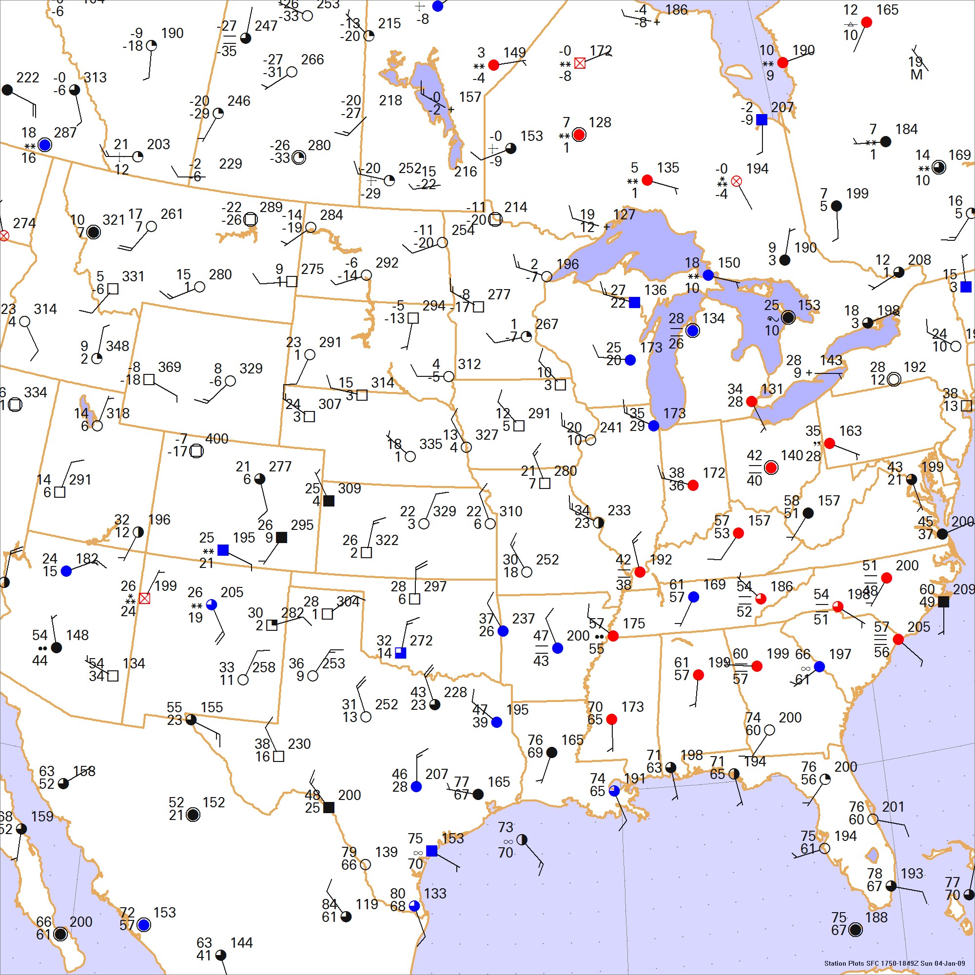
With an abundance of polar air masses, warm ocean temperatures, and a jet stream at its most southward seasonal position, January is full of meteorological action in the United States. In this puzzle readers will find cold fronts, warm fronts, occluded fronts, and several low and high pressure areas. The chinook wind also makes a special guest appearance in the northern Great Plains. Can you find these weather features?

This weather map is an event during the midday hours of January. Draw isobars every four millibars (996, 1000, 1004 mb, etc) using the plot model example at the lower right as a guide. As the plot model indicates, the actual millibar value for plotted pressure (xxx) is 10xx.x mb when the number shown is below 500, and 9xx.x when it is more than 500. For instance, 027 represents 1002.7 mb and 892 represents 989.2 mb. Therefore, when one station reports 074 and a nearby one shows 086, the 1008 mb isobar will be found halfway between the stations. Then try to find the locations of fronts, highs, and lows.

Click to enlarge

* * * * *

Scroll down for the solution

* * * * *

PART TWO: The Solution

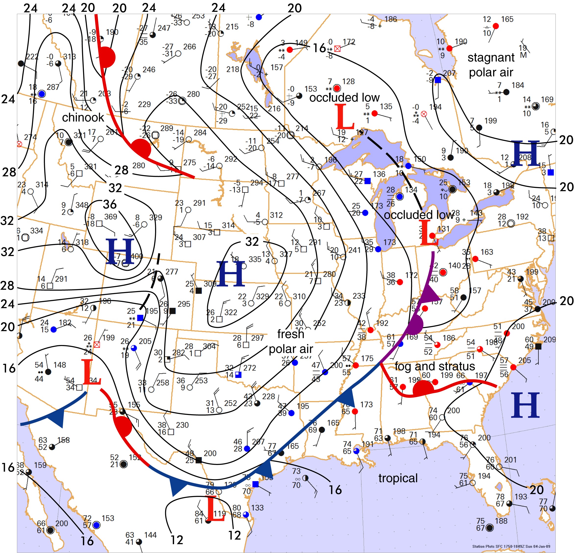
The weather analysis for January 4, 2009 showed a major frontal system tracking through the central United States. The front is easiest to find in the Texas and Louisiana area, and for beginners this is probably the best place to start. Winds and temperatures are significantly different through this region, with winds howling out of the north in Oklahoma and north Texas and mild tropical air on the Gulf coast. The cold front is driven by a large polar high centered in Kansas. This type of system is known as a plunging cold air outbreak. It usually reaches Mexico and nearly all of the Gulf of Mexico, though very strong polar fronts are capable of reaching Honduras, Nicaragua, and much of the Caribbean!

The warm front is somewhat harder to pick out, owing to a gradual transition from warm to cold along the east coast. But the "car trip" technique pointed out in previous issues can be used. With this technique, we simply transect an area where the front is using an imaginary car ride. We imagine that the windows are down and we're constantly monitoring the weather that we see and feel. Starting in Florida, we experience sunny skies and balmy mid-70s readings, perfect if we're driving a convertible. This weather continues through much of southern Georgia, but by the time we're in North Carolina, we're having to roll the windows up, because it's foggy and in the mid-50s. Clearly the air mass has changed between southern Georgia and the Carolinas. The cardinal rule of frontal analysis is that the front is always located on the warm side of the transition zone, in other words, once a transition area has been identified, always place the front on the warm edge of the zone.

Where the cold front and warm front intersect is what is called the "triple point". Often a distinct low pressure area is found at the triple point, but not in this example. What we find is an occluded front extending northward through Tennessee, Kentucky, and into Ohio. In the Great Lakes area we find two low pressure areas. These are older frontal lows that have detached from the warm air mass, drifting towards the dying grounds of the Hudson Bay and Labrador Sea areas and fading away. Still, though, they are capable of producing weather and clouds as long as they can be resolved on the maps and satellite imagery. The triple point area of a frontal system is the prime location for new cyclogenesis to occur, so the forecast for Tennessee and the southern Appalachians certainly calls for a period of unsettled weather for the rest of the day.

Astute readers may have picked out the low-pressure area in the Arizona-New Mexico border area. Quite often weak wintertime lows in this area are associated with cutoff lows, disturbances in the upper troposphere that are well south of the jet stream. However in this case, upper-level charts showed that the area was beneath the southern branch of the jet stream. Furthermore while many cutoff lows tend to "stack" vertically with height, with the low being found at the same geographical location at both the lower and upper levels of the troposphere, the upper-level low in this example was found in the San Diego, California area. This indicates that the Arizona low is a frontal system associated with the jet stream, so fronts can be expected to be found on the chart.

Finally we see an instance of the chinook wind in Montana and Alberta. Here westerly winds are displacing an old polar air mass, replacing subzero temperatures with teens and twenties as Pacific air moves downslope from the Rockies, compresses, and warms. Some of the most dramatic temperature swings in North America are associated with chinook winds, such as on January 14-15, 1972, when a station near Great Falls, Montana rose from -54캟 to 49캟 in only 23 hours!

Computer programs do not produce the Forecast Center solutions. The weather chart is created with Digital Atmosphere, then fronts and isobars are added with Adobe Illustrator.