Forecast Center

May/June 2009

by TIM VASQUEZ / www.weathergraphics.com

This article is a courtesy copy placed on the author's website for educational purposes as permitted by written agreement with Taylor & Francis. It may not be distributed or reproduced without express written permission of Taylor & Francis. More recent installments of this article may be found at the link which follows. Publisher's Notice: This is a preprint of an article submitted for consideration in Weatherwise © 2009 Copyright Taylor & Francis. Weatherwise magazine is available online at: http://www.informaworld.com/openurl?genre=article&issn=0043-1672&volume=62&issue=3&spage=70.

PART ONE: The Puzzle

The Pacific Northwest is often associated with fog and dreary weather, but in fact it's a region full of activity and sudden change. A great many weather systems that reach the central and eastern United States have their roots in the Pacific Northwest, so a prudent forecaster will have a working knowledge of weather systems approaching from this area and be able to monitor how they've evolved.

For this issue's puzzle, at least two major frontal systems will be found: one easy and the other difficult. To locate them, stick to the basics. Use the principle of greatest temperature contrasts to estimate frontal positions, refining them based on troughs, wind shift lines, and other air mass contrasts. There are a few high-altitude stations on this map, so avoid being fooled by their cool temperature readings. Start out with light annotations in pencil, erase them as necessary, then harden in the details once you're confident of the big picture.

This weather map is an event during the early evening in March. Draw isobars every four millibars (996, 1000, 1004 mb, etc) using the plot model example at the lower right as a guide. As the plot model indicates, the actual millibar value for plotted pressure (xxx) is 10xx.x mb when the number shown is below 500, and 9xx.x when it is more than 500. For instance, 027 represents 1002.7 mb and 892 represents 989.2 mb. Therefore, when one station reports 074 and a nearby one shows 086, the 1008 mb isobar will be found halfway between the stations. Then try to find the locations of fronts, highs, and lows.

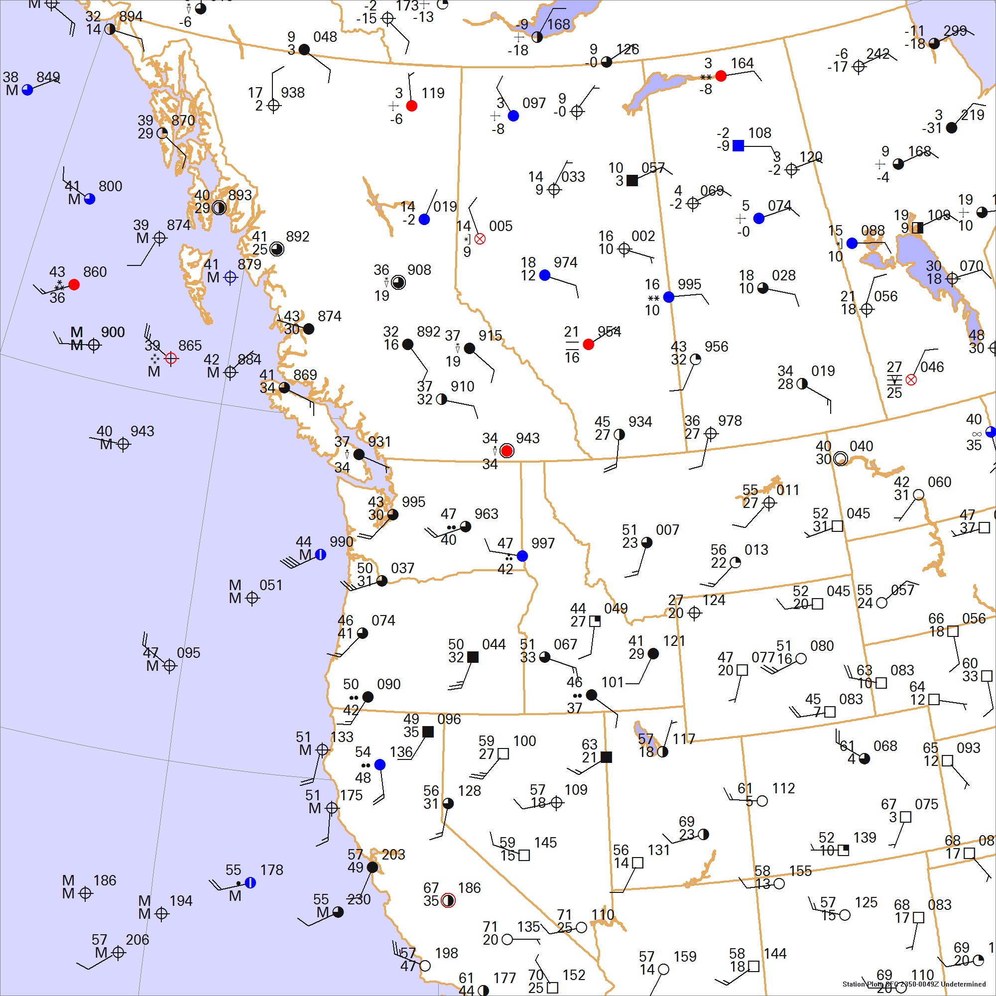
Click to enlarge

* * * * *

Scroll down for the solution

* * * * *

PART TWO: The Solution

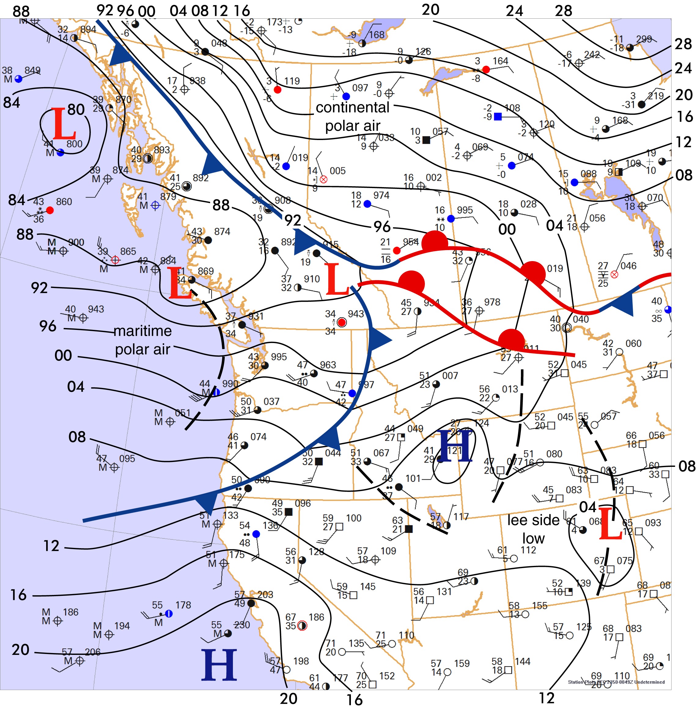
This is perhaps the most challenging map run by Forecast Center in recent years, and it goes to show that Pacific Northwest weather is not comprised of easy, textbook situations. The analysis may require a lot of erasing and redrawing of isobars and fronts to get them just right. If this happens to you, it's normal! It should not raise disappointment but rather reveal that you're paying attention to detail and striving for an accurate conceptual picture of what you see. Adjusting the analysis is a normal process in mentally synthesizing the data and building consistency between all the observed elements. The solution shown here looks deceptively simple but it, too, is the result of numerous changes and adjustments by the author as it was drawn out with illustration software and evaluated.

One aspect of this puzzle that makes it difficult is the presence of mountains throughout the western United States and Canada. This demonstrates the value of having terrain-based relief maps at the forecast desk. A strong polar air mass was positioned in northern Canada, creating very cold conditions in Alberta and Saskatchewan, but this air mass was dammed by the Rocky Mountains in British Columbia. Many polar air masses like this one have a depth of only a few thousand feet, which is not sufficient to ascend into the mountainous terrain and move over mountains and through passes. As a result, much of British Columbia shows southeasterly winds and temperatures above freezing. The front is unlikely to move much further southwest into British Columbia without an unusual depth of cold air and some degree of northerly flow aloft to help move it along.

Astute readers will notice the counterclockwise twist to the wind field near northern Vancouver Island. This hints at the presence of a low pressure system. Indeed the reading of 986.9 mb at Port Hardy, the station at its northern tip, is the lowest pressure in the region. The position of the low is of course not right over Port Hardy but is presumably in the vicinity. We can find it using Buys Ballot's Law. This states that if the wind is at our back in the Northern Hemisphere, the low pressure center will be found to our left. Using this principle at Port Hardy, it can be determined that the low will be found southwest of the station, as drawn in the solution. The isobars should be adjusted around the low to fit it and help locate it properly, also as shown.

Perhaps the most difficult feature to find on the map is the frontal system moving inland through Washington, Idaho, and Oregon. This shows very weak temperature contrasts, further compounded by the greatly-varied altitude of stations inland, particularly in Idaho. Weather forecasters sometimes use a field known as potential temperature, or theta, to help normalize the temperatures across the region to a single common level. When available from websites and software, this can help track fronts in mountainous areas.

In this example, the front can be found only by noticing the difference between the 40-degree temperatures in Washington and Oregon and the 50s in Nevada and the valleys of Idaho, by noticing the slight wind shift, and refining the isopleth analysis to find a pressure trough that might contain it. Conditions in the terrain-free Pacific Ocean can also be used for a first guess. The cool northwesterly wind off the southern Oregon coast contrasts markedly with mild southwesterly winds off the California coast, suggesting the front is in between.

Though it's not part of the Forecast Center puzzle, the single most important element technique for keeping tabs on weak fronts and systems moving through mountains areas is monitoring hourly trends across the forecast region. Sometimes the front will be impossible to find on the weather maps, but a wind shift at Albuquerque, the appearance of showers in Elko, or a decrease in the dewpoint at Boise can uncover its passage. Hourly trends help build a four-dimensional picture of the weather, showing changes over time. These meticulous methods are underrated in the eastern U.S. where forecasters grow accustomed to prominent weather changes. But there, it's the weak weather systems that often make the difference between a blown forecast and spectacular success.

Computer programs do not produce the Forecast Center solutions. The weather chart is created with Digital Atmosphere, then fronts and isobars are added with Adobe Illustrator.